Re-sampling with correlation

Thank you to my colleague and friend Ahmet Balcioglu for his feedback on this post! I also used Anthropic’s Sonnet 4.5 and OpenAI’s GPT-5 to brainstorm ideas for how to solve the problem.

Recently, as part of my research effort to replicate and understand the SHIFT method from the Sparse Feature Circuits paper by Marks et al, I found a way to create custom datasets with specific Pearson correlation coefficient between two binary labels. The aim of the blog post is to show you how I did it in a friendly and accessible way, and to give some intuitions about Pearson correlation coefficients for binary variables!

The Problem Setup

The problem has three inputs:

• A dataset $\DD$ and with two binary labels $X \in \{0,1\}$ and $Y \in \{0,1\}$
• A desired correlation coefficient $-1 \leq \rho \leq 1$
• A desired number of samples $n$ for the output dataset

and a single output:

• A dataset $\dd$ of size $n$ made up of samples from $\DD$ and where the $X$ and $Y$ labels have a Pearson correlation of $\rho$

Additionally, since I want to use $\dd$ to train machine learning models, I want it to have the following properties:

Property 1: Samples in $\dd$ should be independent and identically distributed to ensure that any statistics or machine learning models trained on the dataset are valid.

Property 2: There should be a roughly equal number of samples in each class for both $X$ and $Y$ to avoid arbitrary class imbalances influencing the performance of my machine learning model. In other words, I want that in $\dd$:

The Method

Since we’re dealing with a population with two binary labels, we can think of it in terms of four distinct sub-populations where each sub-population is defined by a particular combination of $X$ and $Y$. We can visualise the sub-populations for the input dataset $\DD$ as a contingency table:

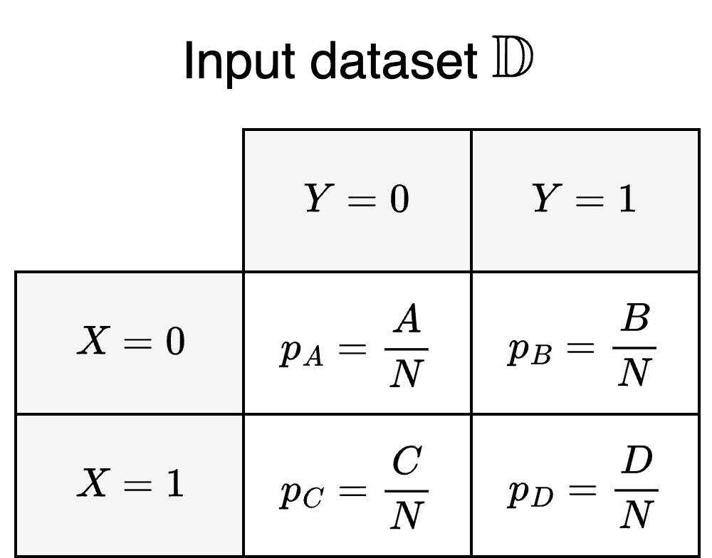
where:

• Each cell represents the sub-population for a particular label pair
• $A$, $B$, $C$, and $D$ are the number of samples in each sub-population
• $N = A + B + C + D$ is the total number of samples in the population
• $p_A$, $p_B$, $p_C$, and $p_D$ are the estimated probabilities for belonging to a particular sub-population

The population defined by $\DD$ will also come with a set correlation between the $X$ and $Y$ labels which we do not control. We can use the following formula to approximate it based on the estimated probabilities of the sub-populations:

This is also known as the Phi coefficient and corresponds exactly to the Pearson correlation coefficient between two binary variables. Note that we could also directly used the sizes of the sub-populations rather than the estimated probabilities and reached the same result, since the factor of $1/N$ in the estimated probabilities cancels out.

If we didn’t care about the correlation between $X$ and $Y$ in the output dataset $\dd$, another thing we could do is to resample $\DD$ to create a new population from the same population distribution. Resampling is a common and widely-used technique to create confidence intervals (bootstrapping) or to validate machine learning models (cross-validation).

Since the sub-populations defined by $X$ and $Y$ are partitions, meaning that every member of the population belongs to one and only one sub-population, we can use stratified sampling to resample the population. To draw a new sample, we first choose one of the sub-populations based on the estimated probabilities, and then draw a sample from within the chosen sub-population uniformly at random. We can then repeat this process $n$ times with replacement to create the resampled dataset. Sampling with replacement here is important to guarantee Property 1, as otherwise the probability of drawing a sample would depend on previously drawn samples. This could result in drawing the same sample more than once in the resampled population, but a few repeated samples are typically not a big issue when training machine learning models so this is OK for our purposes.

More importantly, however, resampling in this way will lead to populations with the same correlation coefficient as $\DD$, which is not what we want. Instead, our goal is to create a new dataset where $X$ and $Y$ have any pre-determined correlation! To achieve this, we have to engineer a new population distribution where the labels have the correlation we desire and which we can sample from using the sub-populations from our original population. In our case this amounts to changing $p_A$, $p_B$, $p_C$ and $p_D$ to some new $p_a$, $p_b$, $p_c$ and $p_d$ based on the desired correlation, and then using the same resampling method as before with the new probabilities. But how should we modify the probabilities?

Lets start simple: what happens if we set all the sub-population probabilities to be the same? Since probabilities have to sum to 1 we have to set them to:

and we get the following correlation in the resampled population:

In this case, since we’ve perfectly balanced the probabilities between each sup-population, the two terms in the numerator cancel out to give us a correlation of 0, which implies that the $X$ and $Y$ labels are linearly independent in the resampled population. If we want to introduce arbitrary correlation we therefore need to skew the probability mass into one of the two terms.

A natural next question is then: what happens when we concentrate all the probability mass into one of the two terms? For instance, we could allocate all the probability mass into the $p_a p_d$ term. Then, we could allocate the probabilities like so:

and we get the following correlation:

Conversely, we could allocate all the probability mass to the $p_b p_c$ term. This means setting the probabilities to:

and results in the following correlation:

Intuitively, this makes sense. $p_a$ and $p_d$ are the probabilities for the sub-populations where $X = Y$, so if samples can only come from those two sub-populations then $X$ and $Y$ in $\dd$ will be exactly the same and exhibit a correlation of 1. Similarly, $p_b$ and $p_c$ are the probabilities for the sub-populations where $X \neq Y$, so if samples can only be selected from those sub-populations then $X$ and $Y$ in $\dd$ will have a perfect negative correlation of -1.

From this, we can conclude that to get an arbitrary correlation in $\dd$ we somehow need to balance the probability mass between the two groups of probabilities. To do this, we can imagine starting from equal probabilities and then symmetrically adding some amount to $p_a$ and $p_d$ and taking the same amount away from $p_b$ and $p_c$. We can do it like this:

where $\delta \in \RR$ and $-1 \leq \delta \leq 1$, since probabilities have to be between 0 and 1. This is nice because it guarantees that the probabilities add up to 1 and that Property 2 holds:

Substituting our values into the Phi coefficient formula we can find the following relationship:

Neat! In order to design a new population distribution with a particular correlation $\rho$, all we need to do is to set:

and the use stratified sampling on the original population with the new probabilities. Note however that for this method to work we need there to be samples in each sub-population in the original population to sample from.

An Implementation

Here’s an example for how to implement the algorithm in Python:

import numpy as np
import pandas as pd

def resample_correlated(
    data: pd.DataFrame,
    correlation: float,
    num_samples: int,
) -> pd.DataFrame:

    msg = f"Correlation {correlation} should be between 0 and 1"
    assert -1.0 <= correlation <= 1, msg

    A = data[(data["profession"] == 0) & (data["gender"] == 0)]
    B = data[(data["profession"] == 0) & (data["gender"] == 1)]
    C = data[(data["profession"] == 1) & (data["gender"] == 0)]
    D = data[(data["profession"] == 1) & (data["gender"] == 1)]

    probabilities = [
        (1 + correlation) / 4,
        (1 - correlation) / 4,
        (1 - correlation) / 4,
        (1 + correlation) / 4,
    ]

    counts = np.random.multinomial(n=num_samples, pvals=probabilities)

    a = A.sample(n=counts[0], replace=True)
    b = B.sample(n=counts[1], replace=True)
    c = C.sample(n=counts[2], replace=True)
    d = D.sample(n=counts[3], replace=True)

    return pd.concat([a, b, c, d], ignore_index=True)

In this case, we are dealing with a dataset with two binary labels: “profession” (nurse or professor) and “gender” (male or female). We use the number of examples in the sub-populations (counts) rather than the probabilities, and rather than performing one draw at a time we batch the sampling for each sub-population.

If you have feedback or find any mistakes, feel free drop an issue on Github or to email me at nicolas.audinet@chalmers.se